Playing Pong with deep Q-learning

3/8/2019

Introduction

Ever since I saw Deepmind's AlphaGo attain super human performance, I've been fascinated with the applications of machine learning to artificial intelligence. But before there was AlphaGo, there was the deep Q-learning network (DQN), developed by Deepmind (see Mnih et al. #1 and Mnih et al. #2) to master a wide range of Atari games using only the raw pixel values.

To understand deep Q-learning it helps to start with a brief overview of reinforcement learning and (ordinary) Q-learning.

Reinforcement learning

In reinforcement learning an agent (the computer) passes through a sequence of states (think: Atari screens) and in each state the agent has a list of available actions it may take (think: buttons on the Atari controller, although technically button combinations may be allowed). The agent's choice of action determines its next state, or more generally, the probability of moving to each of the next possible states. Further, when moving from state s to state s' via action a, the agent receives a reward, which may be positive, negative, or zero (think: the Atari game score changes). The reward received may depend on s, s', and a. This procedure is continued indefinitely, and the goal of the agent is to maximize its expected future reward. However, the agent does not know a priori what the result of its actions will be.

Reinforcement learning is commonly modeled by a Markhov decision process. In detail, a Markov decision process consists of four pieces of data:

A set of states S.
A set of actions A.
For each state s in S and action a in A, a probability distribution P(s,a)(s') which represents the probability of moving to state s', given that the agent is currently in state s and takes action a.
For each pair of states s,s' in S, and action a in A, a function R(s,a)(s') which represents the expected immediate reward given to the agent upon moving from state s to state s' via action a.

We say that a Markov decision process is finite if S and A are both finite sets. Note that a Markov decision process has the Markhov property: the probability distribution P(s,a)(s') depends only on s and a, and not the previous states that the agent has been in.

Q-learning

Q-learning, introduced by Watkins is a reinforcement learning technique which has been shown to converge to an optimal policy for any finite Markhov decision process, given infinite time and a partly-random action-selection policy (see a proof).

In Q-learning, the agent explores the statespace by repeatedly taking an action and observing its reward and next state, and seeks to determine a quality function Q(s,a) (also called a Q-function) which quantifies the value of taking action a in state s. In the beginning, the Q-function is initialized with arbitrary values (for example, all zeros, or all random numbers). As the agent explores, the Q-function is iteratively updated. When the agent is in state s, takes action a, and observes reward r, the value of Q(s,a) is updated according to

Here, alpha is a number between 0 and 1, called the learning rate, which determines how quickly we change our Q-function based on observed information, and gamma, also a number between 0 and 1, is the discount rate. If the discount rate is less than one, future rewards will be valued less than immediate rewards. The idea here is that due to the agent's limited knowledge, predictions for future rewards are likely to become less accurate the further out they go, and hence, immediate rewards should be given some degree of priority.

Because the agent is operating on limited information, in order to guarantee convergence to an optimal Q-function and therefore avoid getting stuck making suboptimal decisions, it needs to continue to explore. To achieve this goal, it is common to follow an epsilon-greedy strategy: the agent takes a random action with probability epsilon (exploration), and a greedy action (the action that maximizes its predicted future reward) with probability 1-epsilon (exploitation).

Deep Q-learning

A Q-function is a function from S x A to the real numbers, which means that an arbitrary Q-function can be thought of as a table (often called a Q-table) where, for example, the rows are indexed by states and the columns are indexed by actions. If there are #S states and #A actions, storing an arbitrary Q-function is therefore equivalent to storing a table with #S*#A entries. For problems where the statespace is extremely large (such as Atari games), this becomes impractical due to the large number of entries that must be stored. In these situations it is often much more efficient to use a parametric model rather than a Q-table.

The idea behind deep Q-learning, introduced by Mnih et al., is to use a neural network, called a deep Q-network, to compute the Q-values instead of an arbitrary Q-function. More specifically, the network takes the state as input and outputs a prediction for the Q-value of each action. In principal, there could be a separate network for each action, but in practice, a single network whose output layer is the size of the action space is used. This weight sharing makes computations more efficient.

In the beginning, the Q-network is initiated with random weights, which means that its predicted Q-values will also be random. Similar to ordinary Q-learning, the agent explores by repeatedly selecting actions (usually according to an epsilon-greedy policy), and observing its reward and next state. After each observation, the agent then stores the tuple (state, action, reward, next state) in "replay memory" and a training step, analogous to the iterative Q-function update in ordinary Q-learning, is performed.

How does the network learn to accurately predict the Q-value of each action? Because adjacent observations are highly correlated, the network trains by randomly selecting a minibatch of samples from replay memory and performing a gradient descent step. Given a sample from replay memory (s,a,r,s'), we must first define the target Q-value, which I will denote by y. If the action a taken resulted in the game ending, we set y equal to the reward r obtained by the action. Otherwise, we set

where gamma is the discount rate (a number between 0 and 1), Q(s',a') is the network's predicted Q-value for taking action a' in state s', and the max is taken over all possible actions a'. We then use a quadratic loss function: if y is the target Q-value for action a in state s, the loss function is

The total loss on each minibatch is then the average of the losses on individual samples above.

One disadvantage of deep Q-learning is that, unlike in ordinary Q-learning, there is no guarantee of convergence to an optimal policy, or even at all. In practice, getting the network to perform well can be tricky, requiring getting a number of hyperparameters to be just right. However, the algorithm has achieved some impressive results.

Playing Atari with a deep Q-network

Mnih et al. aimed to create a network architecture that could be used across a wide range of Atari games. In particular, they sought to avoid using game-specific knowledge as input to the network. Their elegant solution to this problem was to use a convolutional neural network which takes as input only the pixel values displayed on screen.

However, defining the state to be a single gamescreen would not lead to a Markhov decision process. For example, while a single gamescreen likely gives enough information to determine the locations of all in-game objects, it won't give any information about the velocity or acceleration of these objects, and the reward and next state will generally depend on such missing information. To resolve this issue, the deep Q-network takes in the pixel values of four successive game screens. While technically, this still does not guarantee that the Markhov property holds, in practice, on almost all Atari games, it is good enough.

It's worth mentioning here another advantage that the deep Q-network has over a Q-table: the convolutional structure allows the network to recognize common features between different states. Suppose that the agent finds itself in a state that it has never been in before but which differs from a previously experienced state by just single pixel value. When using a Q-table, the agent must learn the Q-values of this new state completely independently from it's knowledge of the other, highly similar, state. When using a convolutional neural network, however, the agent is likely to recognize that it's knowledge of the previously experienced state is relevant to the new state. In practice, this means that in certain situations, the Q-network will converge to an optimal policy much faster than a Q-table.

Network Architecture

Mnih et al. use a deep Q-network with three convolutional layers followed by a hidden dense layer and a dense output layer. The Atari game screen consists of 210x160 rgb pixels. This raw gamescreen is converted to grayscale and cropped and resized to 84x84. Four successive game screens are then stacked together before being fed into the network, so the input to the network is a tensor of shape 84x84x4. The first convolutional layer has 32 filters of kernel size 8x8 and stride 4, the second convolutional layer has 64 filters of size 4x4 and stride 2, and the third convolutional layer has 64 filters of size 3x3 and stride 3. The hidden dense layer has 512 neurons and the last layer has one neuron for each in-game action choice. All four hidden layers use a Relu activation, while the final layer uses no activation since the output of the network represents the Q-value (a real number) of each action for the given input state.

There are a few more important details of Mnih et al's implementation.

To ensure sufficient exploration, the probability of a random action, epsilon, starts at 1 and decreases to 0.1 over the first 1 million frames.
The gamestate is only observed every K=4 frames, and the chosen action is repeated each frame until the next observation. To handle flickering on games such as space invaders, a different value of K, such as 3, can be used, or alternatively, the observed pixels can be set equal to the componentwise maximum of the last two game frames.
Replay memory is capped at a size of 1 million.
Replay memory is filled with 50,000 gameplay observations before training starts.
Rewards are clipped to be between 1 and -1 in order to improve robustness of hyperparameters across multiple Atari games.
Gradient clipping is applied to gradients with absolute value larger than 1.
To aid in convergence and stability, two separate networks are used - a policy network and a target network. The policy network determines the action choice and its weights are trained using gradient descent. The target network is used to compute the target Q-values for the loss function (in my notation above, the value of y). The weights of the target network are not trainable, but rather are set equal to the weights of the policy network every 10,000 frames.
The discount factor is 0.99.
The RMSProp optimizer is used with a minibatch size of 32 and learning rate of 0.00025 (see the nature paper for more details).

Playing Pong

I implemented a deep Q-network using TensorFlow (code on Github), and trained it to play Pong using OpenAI gym. In Pong, the agent and its opponent each control a paddle and attempt to hit a ball past one another. The agent receives a reward of +1 when it scores a point and -1 when its opponent scores a point. The game ends when one of the players scores 21 points total. Therefore, the agent's cumulative reward per game (score) can range from -21 to 21.

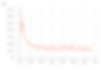
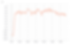
To assess training progress, I sent the following data to TensorBoard every 10,000 training steps: the average loss over the last 10,000 training steps, the average predicted Q-value for the best action choice over the last 10,000 greedy action choices, the average reward over the last 10,000 observation steps, and the average score over the last 100 games. Note that the data is generally pretty noisy, which is typical of deep Q-learning. The score graph is not noisy only because it is averaged over a large number of games, effectively smoothing it out.

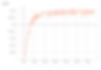
It took a little over 1 million training steps for the network's performance to max out at an average of a 18.24 points per game.

Here you can see the agent (in green) playing against the built-in computer (in orange) before, during, and after training.

My Experience

It was incredibly exciting when I got deep Q-learning to work for the first time. However, I had some false starts on the way, and I found that all the details need to be just right or the algorithm is likely to converge to a suboptimal strategy, or possibly not improve at all. Because training takes a long time even with optimal hyperparameters, experimenting with different settings is time consuming.

There were some technical details of the implementation which have little to do with deep Q-learning per se, but which I found important to getting a good performance. In particular, the default settings in openAI gym cause each action to be repeated for 2-4 frames (chosen randomly) before the next game observation, but these are not the settings used by Deepmind. This issue can be avoided by using the NoFrameskip environments in openAI gym. For pong, use PongNoFrameskip-v4.

Memory optimization is also important. One obvious optimization is to store each observation in memory only once (instead of 4 or 8 times!) and stack them together before inputting to the network. A slightly more subtle point is that while the pixel values should be scaled between 0 and 1 (by dividing by 255) this should not be done before storing in replay memory as this changes the data type from uint8 to float32, which takes up 4 times as much memory. Instead, divide by 255 right before feeding to the network.

Deep Q-learning generally takes a long time to begin to converge to a good policy. Mnih et al.'s goal was to use settings which would be robust enough to work on many different games. However, pong can be mastered faster than other Atari games if different settings are used. To speed up learning on Pong, I eventually settled on the following hyperparameters (similar to those suggested here, with a few details taken from here):

Environment: PongNoFrameskip-v4
Probability of random action: start at 1 and decrease to 0.05 over the first 100,000 frames.
Memory capacity: 10,000
Fill memory with 10,000 observations before beginning training.
Update target network every 1000 frames.
Learning rate: 0.0001
Optimizer: RMSProp (default tensorflow settings other than the learning rate)